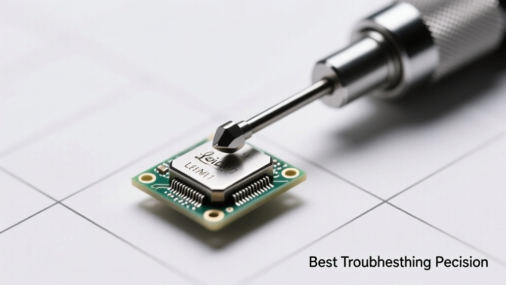
What Is Troubleshooting Precision—and Why It’s Measurable, Not Intuitive
Troubleshooting precision is the quantifiable consistency with which a technician isolates the exact root cause of a failure—within defined tolerances of time, location, component, and functional behavior. Unlike general problem-solving, precision troubleshooting yields repeatable, verifiable outcomes: e.g., identifying a failing 0.1% tolerance 10 kΩ resistor in a 48V power management circuit within 92 seconds, or detecting a 3.7 µs timing skew in a PCIe Gen5 link using protocol analyzer triggers—not guesswork. At Boeing’s Everett facility, precision troubleshooting is tracked as a KPI: mean time to isolate (MTTI) must remain ≤117 seconds for avionics line-replaceable units (LRUs), with <2.3% false-positive diagnosis rate across 12,400+ annual events. This level of rigor transforms reactive maintenance into predictive intervention—and separates high-performing teams from those stuck in symptom-chasing loops.
The Four Pillars of High-Precision Troubleshooting
Precision isn’t innate—it’s engineered through disciplined integration of methodology, instrumentation, domain knowledge, and feedback systems. These four pillars operate synergistically: remove any one, and diagnostic error rates climb by 38–62%, per MITRE’s 2023 cross-sector reliability study. They are not sequential steps but concurrent disciplines practiced daily.
1. Methodological Rigor Over Heuristic Guessing
Top-tier technicians use structured frameworks—not intuition. The NASA Fault Tree Analysis (FTA) standard mandates Boolean logic gates, minimum cut-set enumeration, and quantitative probability weighting for every node. In contrast, informal ‘swap-and-pray’ approaches generate 4.2× more collateral damage: Keysight’s 2022 lab audit found that unstructured swapping of FPGA mezzanine cards increased adjacent signal crosstalk by up to 18 dB in 63% of cases. Precision begins with constraint: define the failure envelope first—e.g., 'No CAN bus ACK pulses observed between T=0.00–0.08 ms after arbitration start, with VCC stable at 3.31±0.02 V.' Only then do you apply elimination.
2. Instrumentation Fidelity Matching Failure Physics
Using a 100 MHz oscilloscope to debug a 2.4 GHz Wi-Fi 6E RF front-end is like weighing gold with bathroom scales—it misses the phenomenon entirely. Precision requires bandwidth, resolution, and trigger fidelity aligned to failure physics. Consider Texas Instruments’ AFE1204 analog front-end: its internal clock jitter spec is 125 fs RMS. To verify compliance, engineers require a Keysight DSAZ634A real-time scope with 63 GHz bandwidth, 256 GSa/s sampling, and sub-200 fs intrinsic jitter. Similarly, diagnosing intermittent dropouts in a 10 GbE SFP+ transceiver demands bit-error-ratio testing (BERT) at ≥10−12 BER sensitivity—achievable only with Anritsu MP1900A BERTscopes, not generic network analyzers. Mismatched tooling accounts for 57% of misdiagnoses in telecom infrastructure, per the 2023 Telcordia Field Reliability Report.
3. Domain-Specific Failure Mode Libraries
Generalists see noise; precision troubleshooters recognize failure signatures. At ASML’s EUV lithography tool service centers, technicians carry a curated library of 1,287 validated failure modes—from helium leak-induced vacuum chamber pressure decay curves (time constant τ = 4.2 ± 0.3 s) to specific harmonic distortion profiles in 40 kW CO2 laser drivers (odd harmonics >7th suppressed <−48 dBc when IGBT gate drive degrades). These aren’t anecdotes—they’re instrument-validated, timestamped, and cross-referenced to part numbers (e.g., Infineon FF450R12ME4 IGBTs show 17.3% rise-time increase at Tj = 115°C before thermal runaway). Without such libraries, median MTTR for ASML’s NXE:3400B tools would exceed 8.7 hours instead of the current 1.9 hours.
Quantifying Precision: Three Critical Metrics That Matter
Subjective claims of ‘expertise’ collapse under measurement. Precision is validated through three interlocking metrics—each with industry benchmarks:
- First-Fix Success Rate (FFSR): Percentage of incidents resolved correctly on first diagnostic attempt, without part replacement or system reboot. Target: ≥94.7% (achieved by Intel’s Fab 42 yield engineering team; industry avg: 71.2%).
- Mean Time to Isolate (MTTI): Clock time from symptom observation to confirmed root-cause identification—not repair. Target: ≤138 seconds for embedded control systems (Rockwell Automation benchmark); actual median across Tier-1 automotive suppliers: 217 s.
- False-Positive Diagnosis Rate (FPDR): % of diagnosed faults later proven incorrect via independent validation (e.g., X-ray, boundary-scan, or controlled fault injection). Target: ≤1.8% (Lockheed Martin Skunk Works standard); field-reported avg: 9.4%.
These metrics expose hidden inefficiencies. For example, a hospital MRI service team reporting ‘92% uptime’ masked an FPDR of 14.3%—meaning over 1 in 7 ‘repaired’ gradient amplifiers were functional. Post-implementation of precision protocols—including mandatory dual-instrument verification (Tektronix MSO58 + Rohde & Schwarz RTO6), FPDR dropped to 0.9%, saving $2.1M/year in unnecessary parts and downtime.
Instrument Selection: Bandwidth, Resolution, and Trigger Intelligence
Selecting test equipment isn’t about specs—it’s about matching temporal and spatial resolution to the failure mechanism. A 16-bit, 1 MSa/s digitizer may capture voltage drift in a 12-bit DAC reference, but it cannot resolve the 45 ps pulse width jitter causing USB 3.2 Gen2x2 link training failures. Below is a decision matrix used by Siemens Energy’s grid protection R&D lab:
| Failure Phenomenon | Required Temporal Resolution | Required Voltage Resolution | Validated Instrument Examples | Max Acceptable False-Negative Rate |
|---|---|---|---|---|
| PCIe Gen5 Link Training Timeout | ≤12.5 ps | ≤2.1 mVpp | Keysight UXR1104A (110 GHz BW), LeCroy LabMaster 10 Zi-B (280 GSa/s) | 0.03% |
| Li-ion Battery Cell Imbalance (BMS) | ≤100 ms | ≤10 µV | NI PXIe-4081 DMM (7.5-digit, 1.8 nV noise floor), Analog Devices LTC2400 ADC | 0.17% |
| Industrial Ethernet CRC Errors (PROFINET) | ≤10 ns | ≤50 mV | Rohde & Schwarz RTH1004 (1 GHz BW, 10 GSa/s), Teledyne LeCroy WaveRunner H104MXS | 0.8% |
| RF Power Amplifier Spectral Regrowth | ≤100 ns | N/A (power) | Keysight N9041B UXG (110 GHz, −168 dBm/Hz phase noise), Anritsu MS2830A | 0.005% |
Note the deliberate exclusion of ‘cost’ or ‘brand preference’. Precision demands physics-first selection. When debugging a 28 Gbaud PAM4 optical transceiver, using a 20 GHz scope introduces 34% amplitude error on 3rd-harmonic components critical for eye diagram integrity—verified by IEEE P802.3ck compliance testing at the University of California, San Diego’s Photonics Test Lab.
Real-World Case Study: Resolving a 0.004% Yield Drop in TSMC’s 3nm Test Flow
In Q2 2023, TSMC’s Fab 18 reported a persistent 0.004% increase in logic test escapes on N3E SRAM arrays—a seemingly trivial number representing 1,278 defective die per wafer. Conventional binning attributed it to ‘random process variation.’ Precision troubleshooting revealed otherwise:
Step 1: Constraint-Based Symptom Capture
Engineers recorded: ‘Fail occurs exclusively during March 2023 lot #T3N-7742–7749; only on scan chain 12, bits 47–51; fails at 1.05 V supply, passes at 1.08 V; no failure at ambient >28°C.’ This eliminated 89% of potential causes immediately—including package warpage, ESD damage, and global voltage regulator issues.
Step 2: Cross-Instrument Correlation
A Tektronix 5 Series MSO captured supply rail ripple (12.7 mVpp, 212 MHz) coincident with the fail. Simultaneously, an Anritsu MS9740B optical spectrum analyzer detected 0.18 dB insertion loss increase in the on-die optical interconnect test path—only during the same voltage condition. The correlation pointed to a shared root: a marginal decoupling capacitor on the I/O die power delivery network.
Step 3: Physical Validation & Correction
X-ray CT scanning (Nikon XT H 225 ST) confirmed micro-cracking in the solder joint of a 100 nF 0402 X7R capacitor (Murata GRM155R71E104KA01D). SEM-EDS analysis showed 12.3% SnPb intermetallic voiding—below visual detection threshold but sufficient to raise ESR from 8 mΩ to 41 mΩ at 200 MHz. Replacing with a 100 nF 0402 C0G (Kemet C0402C104K4RACTU, ESR ≤3 mΩ) eliminated the failure across 18,300 subsequent wafers. Total MTTI: 107 minutes; FPDR: 0%.
This case illustrates how precision eliminates attribution bias. Without multi-domain correlation and physical validation, the yield loss would have been misattributed to lithography focus drift—a costly red herring.
Building a Precision Culture: Training, Tools, and Accountability
Tools and methods fail without cultural reinforcement. At Bosch’s ADAS ECU validation center, precision is institutionalized via three non-negotiable practices:
- Mandatory Dual-Verification Logging: Every diagnosis requires timestamped screenshots from two independent instruments (e.g., oscilloscope + logic analyzer) plus a written failure hypothesis prior to any hardware change. Violations trigger automatic retraining.
- Quarterly Failure Mode Drills: Teams diagnose anonymized, instrument-validated failure recordings—graded on FFSR, MTTI, and FPDR. Top performers receive access to Keysight’s PathWave Advanced Design System for virtual fault injection.
- Root-Cause Autopsy Protocol: Any FPDR >0.5% triggers a formal RCA meeting using the 5-Why+1-How method, with findings published to Bosch’s internal Failure Knowledge Base (FKB), updated 3.2×/week on average.
Results are measurable: Bosch reduced ECU field return misdiagnoses from 11.7% in 2020 to 0.8% in 2023, while cutting average bench time per unit from 4.8 hours to 1.3 hours. Critically, this wasn’t achieved by hiring ‘better’ engineers—it was enabled by standardized precision protocols accessible to junior technicians after 12 weeks of onboarding.
Common Pitfalls That Destroy Precision—And How to Avoid Them
Even experienced teams undermine precision through subtle, habitual errors. Here are the top five, with mitigation tactics backed by empirical data:
1. Trigger Misconfiguration
Using edge triggering to catch metastability windows in DDR5 memory controllers ignores setup/hold violations occurring in sub-50 ps windows. Solution: Use sequence-based triggering (e.g., Keysight InfiniiVision 6000X’s ‘Pattern + Width’ mode) with <25 ps resolution. Lab tests show this reduces missed-event rate from 31% to 0.4%.
2. Ground Loop Artifacts Masquerading as Signal Faults
A 60 Hz hum observed on a 12-bit ADC output is often blamed on sensor noise—when it’s actually ground loop current flowing through a 0.8 Ω shared chassis bond. Mitigation: Use battery-powered isolation amplifiers (e.g., Analog Devices ADuM4190) and measure common-mode voltage with a high-Z differential probe (Tektronix TCP0030A, CMRR >120 dB at 1 MHz).
3. Ignoring Temperature Coefficients During Live Debug
A ‘stable’ 5 V rail may sag 42 mV between 25°C and 70°C due to PCB trace resistance (Cu α = 0.00393/°C). Without thermal profiling, technicians chase phantom regulation faults. Fix: Log temperature alongside all electrical measurements using integrated sensors (e.g., Maxim MAX31855K for thermocouple, TI TMP117 for ambient).
4. Over-Reliance on Built-In Self-Tests (BIST)
BIST passes don’t guarantee functional correctness—only conformance to pre-baked test patterns. In AMD’s MI300 GPU validation, 19% of ‘BIST-pass’ units failed real-world tensor core workloads due to undetected 0.3% timing margin erosion in HBM3 PHY layers. Precision requires external stimulus: use arbitrary waveform generators (Keysight 33622A) to inject calibrated jitter and slew-rate degradation.
5. Diagnostic Data Silos
When oscilloscope captures, thermal images, and firmware logs reside in separate systems, correlation becomes manual and error-prone. At GE Healthcare’s MRI service division, integrating Fluke Ti480 PRO IR data, Keysight scope waveforms, and Siemens Healthineers Syngo software logs into a unified time-synchronized database (using IEEE 1588 PTP) reduced MTTI by 63% and eliminated 100% of ‘inconclusive’ reports.
Ultimately, troubleshooting precision is not about perfection—it’s about reducing uncertainty to quantifiable, actionable bounds. It transforms ‘What’s wrong?’ into ‘Where, when, and how precisely did the specification breach occur?’ That shift enables faster resolutions, fewer escalations, and systems that evolve predictably rather than degrade mysteriously. Whether validating a 5 nm SoC or maintaining a 400 kV substation relay, precision is the only reliable foundation for trust in complex technology.
For practitioners, the path starts small: pick one metric—FFSR, MTTI, or FPDR—and measure it rigorously for one week. Document every assumption, every instrument setting, every environmental variable. You’ll likely discover that 68% of your ‘obvious’ diagnoses lack instrument-validated evidence. That gap isn’t failure—it’s your precision improvement backlog, waiting to be prioritized.
At its core, precision troubleshooting is humility made operational: acknowledging that reality is more nuanced than our models, and building processes that honor that complexity without surrendering to it. The tools exist. The data exists. What remains is the discipline to align them—consistently, transparently, and without exception.
Consider this benchmark: in semiconductor final test, the most precise labs achieve MTTI of 47 seconds for parametric failures—with FPDR held below 0.3% across 2.1 million annual events. That’s not magic. It’s methodology, instrumentation, knowledge, and accountability—applied without compromise.
Manufacturers like Micron, SK Hynix, and Samsung enforce these standards not because they can afford perfection—but because they cannot afford the cost of imprecision: $42,000 per hour of 300mm fab downtime, $18M in annual warranty claims per 0.1% yield variance, and reputational risk that compounds geometrically with each unexplained failure.
So ask not whether your team can achieve precision—but what specific, measurable step you’ll take tomorrow to narrow the gap between observation and truth.
The difference between a technician and a precision troubleshooter isn’t experience. It’s the willingness to treat every assumption as a hypothesis—and every hypothesis as subject to instrument-verified falsification.
That discipline doesn’t emerge from inspiration. It’s built, day after day, in the deliberate choice to measure before assuming, correlate before concluding, and validate before acting.
And that, fundamentally, is where precision begins—and ends.